Whether a professional or amateur, one of the first things we learn about propagation is that lower frequencies propagate better. Or propagation loss increases with frequency. In this post I will make the case that Free Space Path Loss really does not exist, and that the real effect we see is independent of frequency.

How can this be so you say. I know my HF HAM radio can transmit for hundreds of miles, yet I can’t receive my WiFi at the bottom of the garden. Ignoring the fact that WiFi data rates are vastly larger than FM voice that our friend Claude Shannon will tell you requires more energy, trust me, WiFi would have shorter range than HF voice even if the data rates were the same.

So let’s square away my statement that true Pathloss does not depend on frequency with our lived experience.

Our sun is a ball of light that shines in all directions. It emits electromagnetic waves(light) that illuminate all the planets in our solar system. The further a planet is from the sun, the dimmer the light that reaches it. Why is this so? It’s clearly not because of dust in space that is absorbing this light and turning it into heat, such an effect would cause the dust to emit black body radiation(probably IR light) and the sky would glow(at least in IR) which it doesn’t. No, the light gets dimmer because it spreads out as it travels. If we placed a huge sphere around our solar system (Dyson sphere) pretty much all the light emitted from the sun would be hit the inside surface of that sphere. Note, that I haven’t had to discuss the colour or frequency of this light. It does not matter.

The same is true for a radio signal. Within the air of our atmosphere and within the frequencies we normally deal with for radio signals, air is pretty much a lossless medium. We will ignore some effects like hydrogen lines and water absorption that happen in specific bands. Regardless, my argument here is about Freespace Pathloss, so let’s assume we are in a vacuum. There is no Loss in a vacuum, if there were we would not be able to see the stars. Hence Freespace Pathloss does not depend upon frequency.

But above is the Freespace pathlos formula Mr HexAndFlex, it clearly has a frequency term! What is going on? Well I will try and avoid too much math here, but unfortunately some is essential.

Let us first understand that the freespace pathloss formula is derived from this basic principle. In the formula above(fig2), we show the transmitted power in the numerator(above the line). In the denominator, we see what is clearly recognisable as the formula for the surface area of a sphere. The intensity of the signal decreases as the surface area of a sphere of radius d(yes, I know radius is normally r, but for some reason RF people use d to equal distance). There is no loss, but the power density, which would have units like Watts per Meter Squared, decreases according to the size of the sphere. This in my opinion really is the fundamental formula we should understand. Its not complicated, and very easy to intuitively understand.

So, why does our FSPL formula differ from this. Well its because of the way we specify antenna gain. For good reasons, we do this in a way that similar similar antennas provide the same gain when scaled for frequency. A standard half-wave dipole will have a gain of 2.15dBi regardless of frequency. Our dipole is tuned to a specific frequency that we can change by making it shorter or longer. If we want to make our antenna work at a higher frequency we make it shorter. The power intensity we calculated in fig2 is in units of W/m^2, ie. Watts per Unit Area, it stands to reason that if the Area is smaller(because our antenna is shorter) there will be less received power.

Formulas in fig1 and fig2 are different because the FSPL formula has the assumption of an isotropic antenna built in.

This brings me to what I think is the real understanding of the link between FSPL and frequency. Freespace Pathloss increase with frequency because our antennas get smaller. In fact to call it a ‘loss’ is somewhat confusing. Nothing is lost, we are just using a smaller bucket to catch the signal with.

If we can design an antenna such that its size remains the same with increasing frequency, we can compensate for this loss. This is true for a type of antenna called an ‘aperture antenna’. A common example of which would be a satellite dish. So long as the wavelength is smaller than the area of the dish, these antennas work to capture all the energy that hits the dish. It has a constant aperture, dictated by the diameter of the dish. Assuming its 100% efficient(dishes are normally at least 70% efficient). We can calculate this aperture(area of the dish) and multiply if by the power intensity(fig2), we can work out the received power.

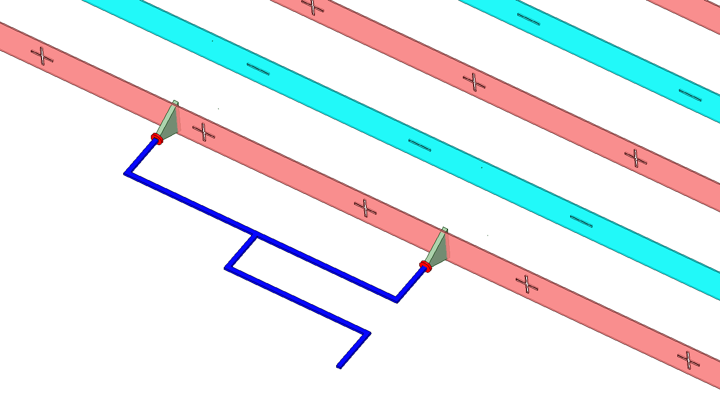
For my Palmtree Vivaldi antenna, I did a similar calculation. As a planar antenna, its hard to easily see what the aperture is, but given a bit of experimentation I was able to derive a suitable area that worked for my needs. In the diagram below I have drawn a cyan rectangle to represent the assumed aperture for my antenna(45cm^2). Assuming this was fixed, I calculated the calculated the expected gain that this would result in.

In the above plot, we can see that the blue gain(dBi) and red fixed aperture gain plots show very good correlation. There would be very little point in trying to optimise this antenna any further to enhance gain, unless we are willing to try and increase the aperture(and hence size).

Summing up

Firstly, to get it out of the way. The standard FSPL formula is correct and within the system we tend to work with where we calculate our antenna gains with respect to a isotropic antenna, it is a useful way to calculate link budgets etc. Please don’t read this post and think that antenna theory is really built on a lie and you need to throw away your books. However hopefully this post provides another viewpoint that may give you greater insight into why things work the way they do.

The terminology of FSPL somewhat misleading in my opinion. We do not loose energy because the there is some ‘loss’ along a path. The energy is lost, because some of it has traveled down a different path that no longer leads to our antenna. It is still there should we place more antenna in its way to receive it.

I have been careful in this post to only discuss things in freespace(i.e. a vacuum). when we start to add real world materials into the mix, things definitely diverge from this. House bricks definitely do increase the loss of signals that pass through them and this loss is very much dependent upon frequency, although not necessarily in a way that can be easily inserted into such a simple mathematical formula. However, when we start to think about propagation in environments that contain significant other materials, FSPL is probably not the way we want to estimate pathloss.